SLAM

Simultaneous Localization and Mapping (SLAM) is the process of estimating a vehicle’s position and orientation while simultaneously building a map of its surrounding environment. This is useful when an accurate pre-existing map or global position is unavailable. Since SLAM relies on revisiting landmarks to correct accumulated localization drift, it is most effective on events with multiple laps, such as Trackdrive. Offline SLAM can also be used to validate the track and localization data of a run by comparing the generated map and trajectory against the expected track layout.

SLAM combines odometry from IMU data with environmental observations from sensors such as LiDAR or cameras. Motion measurements provide an estimate of how the vehicle moves, while observations of known or previously seen landmarks provide information that can correct accumulated drift.

As the vehicle moves, SLAM continuously estimates:

• Vehicle pose: the vehicle’s position and orientation.
• Landmarks: the locations of identifiable objects in the environment.
• Data associations: which observations correspond to previously mapped landmarks.

The system uses these measurements to find a trajectory and map that are jointly consistent with the available sensor data. Reobserving landmarks is particularly important because it allows SLAM to detect and correct accumulated localization drift.

SLAM Approaches

EKF-SLAM

EKF-SLAM formulates SLAM as an Extended Kalman Filter problem, maintaining a single joint Gaussian estimate over the vehicle pose and all landmark positions. As new odometry and cone measurements arrive, this joint estimate is updated recursively through the EKF predict/update cycle, linearizing the motion and measurement models around the current estimate at each step.

This approach has two limitations that motivated our choice of graph-based SLAM instead:

• Scalability. The EKF’s state covariance matrix grows quadratically with the number of landmarks, making each update more expensive as the cone map grows — a concern given the large number of cones observed over a multi-lap event.
• Linearization. EKF-SLAM linearizes around the current estimate once per step and does not revisit that linearization later. If an early pose or landmark estimate is inaccurate, that error is not easily corrected. Graph-based SLAM instead keeps the full history of poses and landmarks as nodes in the factor graph, allowing iSAM2 to incrementally relinearize and adjust past estimates as new, more accurate information arrives.

For these reasons, we selected graph-based SLAM, described below, over EKF-SLAM for this implementation.

Graph-Based SLAM

Graph-based SLAM models the problem as a network of nodes (representing robot poses or landmarks) connected by edges (representing spatial constraints or sensor measurements).

Factor Graph

The factor graph contains two types of variables:

• Vehicle poses ($x_n$): the vehicle’s position and heading at each timestep.
• Cone landmarks ($l_n$): the estimated global position of each observed cone.

Factors encode constraints between these variables. The optimizer then finds the set of poses and landmark positions that best satisfies all of these constraints.

Note

A Variable Node cannot be adjacent to another Variable Node, and a Factor Node cannot be adjacent to another Factor Node. Blue nodes represent Variable Nodes: $x$ variable nodes represent car poses, while $l$ variable nodes represent landmark positions. Gray nodes represent Factor Nodes. Factor Node $f_0$ is a Prior Factor node, anchoring the first pose (and, in some cases, the first landmark) to establish a reference frame for the SLAM system as it estimates future poses and landmarks.

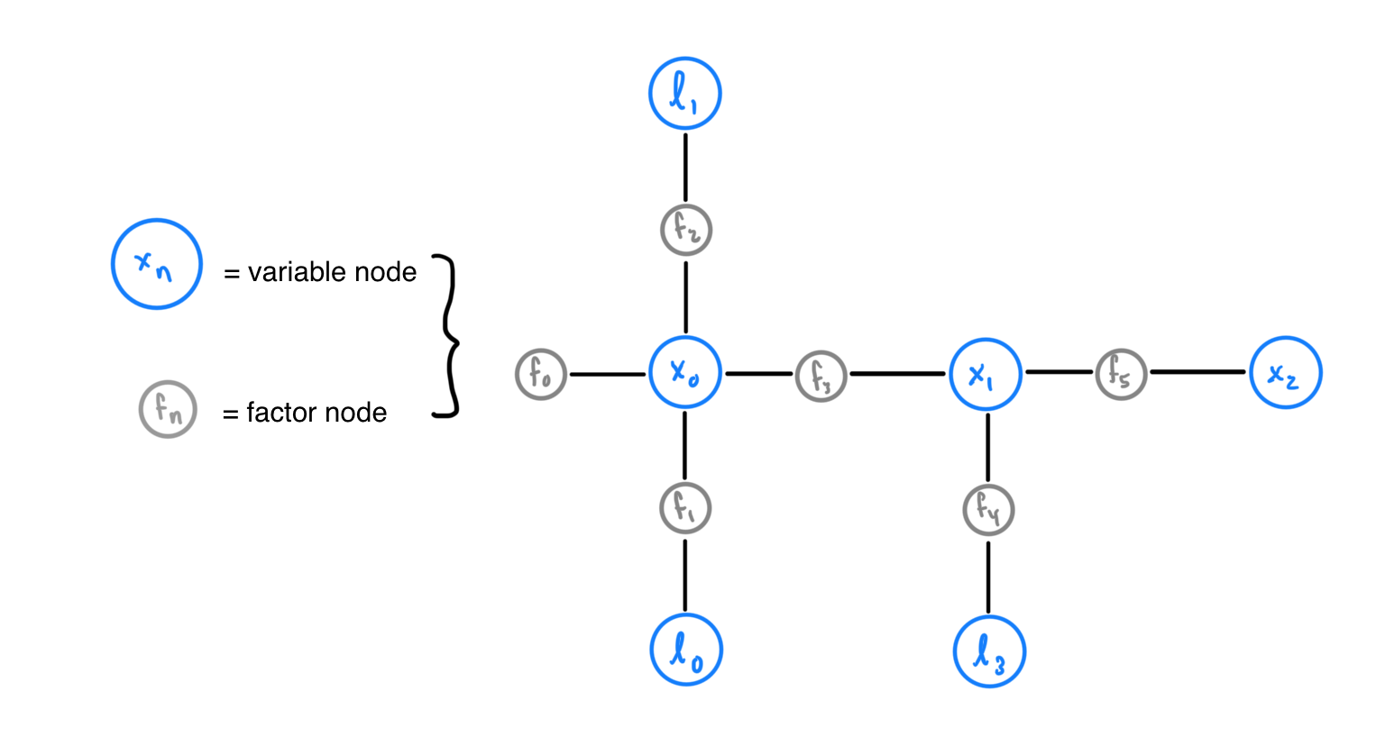
For example, in the factor graph above, Factor Node $f_1$ is connected to Variable Node $x_0$, representing the first car pose, and $l_0$, representing the first landmark. The factor represents a probabilistic constraint relating the estimates of $x_0$ and $l_0$ based on the corresponding measurement and its uncertainty.

The complete Factor Graph combines these individual factors into a joint probability distribution over the vehicle poses and landmark positions. The SLAM system then finds the pose and landmark estimates that best satisfy the constraints represented by the factors.

Vehicle Pose Factors

We use odometry to get the estimated pose from the linear and angular velocity measurements of the twist topic. The resulting relative motion is added to the graph as a vehicle pose factor between consecutive vehicle poses. The uncertainty of the odometry is represented by the factor’s noise model, allowing the optimizer to adjust the trajectory when cone observations provide contradictory information.

Landmark Position Factors

Each detected cone provides a relative position measurement from the vehicle. After associating the observation with a landmark, the system adds a factor connecting the current vehicle pose to that landmark. This constraint compares the measured cone position with the position predicted from the vehicle pose and landmark estimate, allowing the optimizer to jointly refine the trajectory and map and correct accumulated odometry drift.

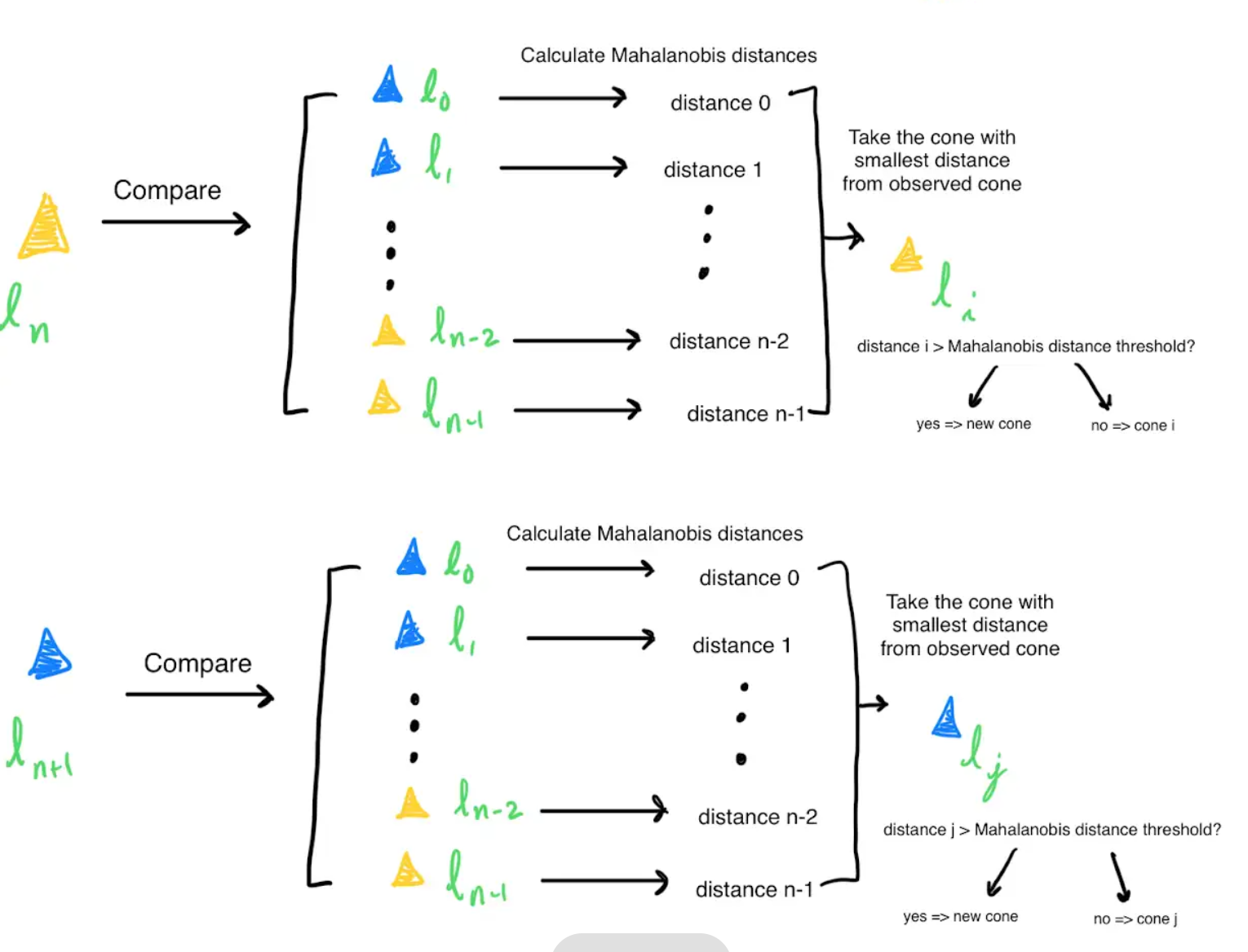
Data Association

Before adding a cone observation to the factor graph, the system attempts to determine which existing landmark corresponds to the observation. If an observation matches an existing landmark, a landmark position factor is added between the current vehicle pose and that landmark. If no suitable landmark is found, a new landmark is initialized and added to the graph. This process is repeated for every cone batch in the recorded data.

Mahalanobis Distance

To perform data association, the Mahalanobis Distance is calculated between an observed cone and all iSAM2 estimates for previously seen cones. Unlike Euclidean distance, which only measures the distance between two points, Mahalanobis Distance accounts for the uncertainty in the landmark’s estimated position — effectively measuring the distance between a point and a distribution rather than between two points (see more).

If the smallest distance is greater than the Mahalanobis Distance Threshold, the observed cone is considered a new cone.

Tip

The Mahalanobis Distance threshold is generally found through tuning and trial and error.

iSAM2 Optimization

After adding the new factors and variables, the graph is optimized using iSAM2 (Incremental Smoothing and Mapping), an incremental nonlinear optimization algorithm provided by the GTSAM library. Rather than recomputing the entire solution from scratch for every observation, iSAM2 incrementally updates the existing solution as new measurements arrive.

The optimization balances:

• consistency with the vehicle’s odometry
• consistency with cone observations
• consistency between repeated observations of the same landmarks

As a result, the estimated vehicle trajectory can deviate from the raw odometry when the cone observations provide evidence that the vehicle has drifted.

Why iSAM2?

We chose this algorithm after considering:

1. Incremental updates. iSAM2 incrementally re-optimizes previous cone position and pose estimates as new data arrives, rather than only optimizing at loop closure like some batch approaches.
2. Performance. iSAM2’s performance made it a clear choice for SLAM. Our iSAM2 SLAM implementation runs entirely on the CPU. It is written in C++ and uses GTSAM, a CPU-optimized factor graph library. No GPU acceleration is needed, since iSAM2’s incremental updates are efficient enough for real-time execution on modern multi-core CPUs. Our SLAM nodes run within a ROS 2 node written in C++ and leverage threading where available (through TBB), although much of the computation remains serial due to the incremental nature of the updates.
3. We were able to work closely with the author of iSAM2, Professor Michael Kaess. Thus, we would like to take this opportunity to thank Professor Michael Kaess for dedicating his time and efforts to assisting our implementation of SLAM.

Implementation

The iSAM2 node first parses the cones received by perceptions into separate vectors by color. This vector of observed cones and other odometry information is used to update the iSAM2 model as well as the car’s current pose.

A Variable Node $x_n$, representing the car pose at the current timestamp, is added alongside a Factor Node connecting $x_n$ to $x_{n-1}$, the Variable Node representing the previous car pose.

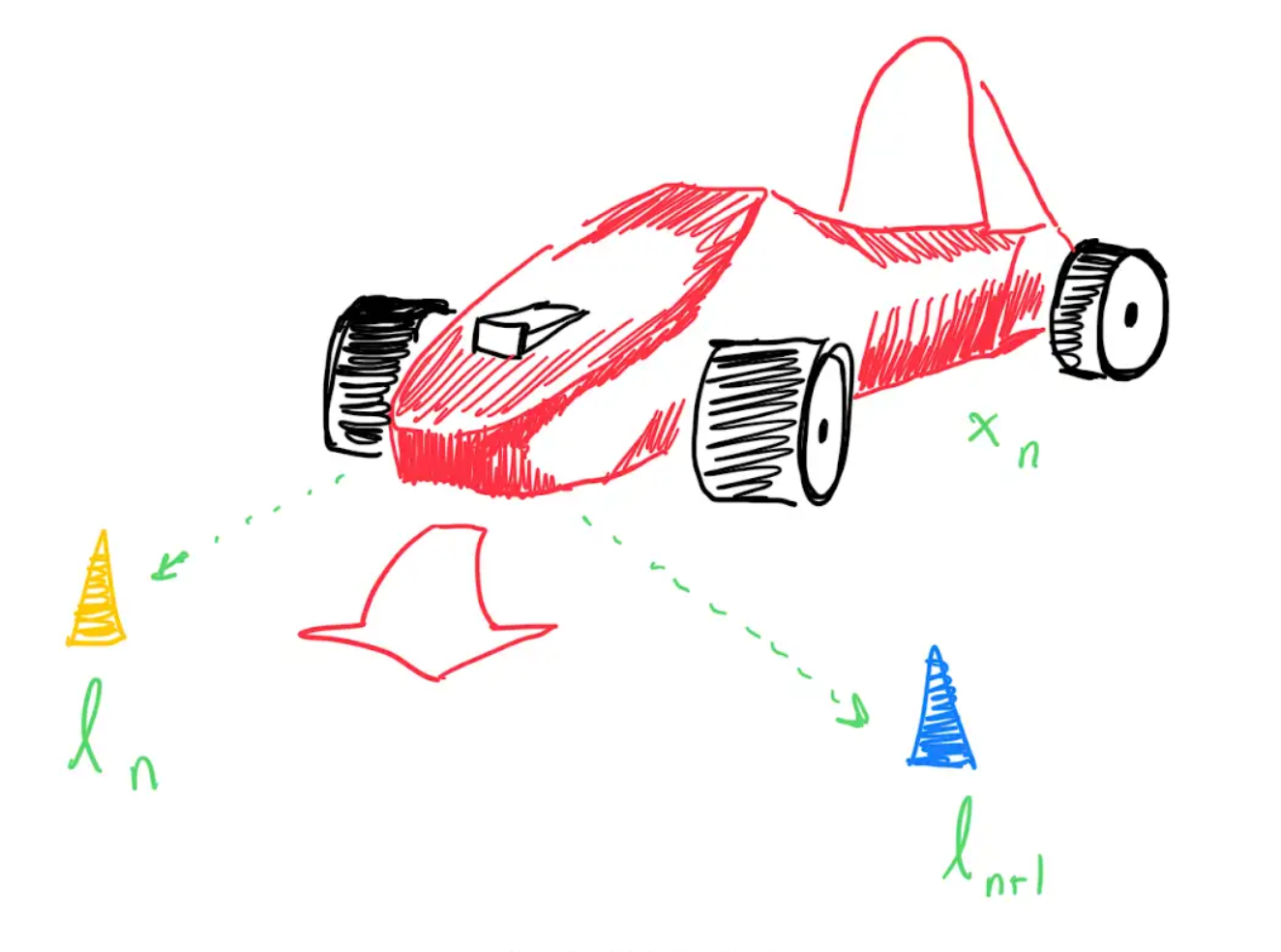
After determining the car pose, Data Association is performed on the cones observed at the current timestamp to determine which of the observed cones are new.

For each observed cone, the Mahalanobis Distance is calculated between the observation and the iSAM2 estimates for previously seen cones. If the smallest distance is below the Mahalanobis Distance Threshold, the observation is associated with the corresponding existing landmark. Otherwise, a new landmark is initialized.

Each detected new cone is added to the Factor Graph as a Variable Node with a Factor Node connected to $x_n$, the Variable Node representing the current car pose.

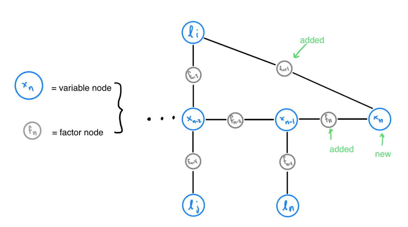
This process is repeated for all observed cones. After the new variables and factors have been added, iSAM2 incrementally optimizes the graph and updates the estimated vehicle trajectory and landmark positions.

Online SLAM

The online SLAM system runs the same factor graph pipeline described above, but processes vehicle motion and cone observations in real time as they are published by the perceptions and odometry nodes during a run, rather than replaying a recorded ROS 2 bag.

Because online SLAM runs continuously during a run, it is especially effective on multi-lap events like Trackdrive, because as previously seen cones are reobserved on later laps, iSAM2 corrects accumulated drift in the trajectory and map in real time. See the Workflow Comparison below for a side-by-side view of the online and offline pipelines.

Offline SLAM

The offline SLAM system reconstructs the vehicle trajectory and a map of the surrounding cones from recorded ROS 2 data. It follows the same factor graph pipeline as online SLAM, but replays a recorded ROS 2 bag instead of processing live sensor measurements.

Offline Validation

Offline SLAM can be used to validate both localization and perceptions data from a recorded run. The generated trajectory can be compared against reference localization data, while the generated cone map can be inspected for incorrect associations, duplicate landmarks, and other mapping errors.

This allows us to evaluate SLAM and tune its parameters without requiring the vehicle to be running.

Workflow Comparison

Online and offline SLAM share the same core pipeline — data association, adding vehicle pose and landmark position factors to the factor graph, and incremental optimization with iSAM2. They differ only in where the data comes from and what happens to the result:

	Online SLAM	Offline SLAM
Data source	Live vehicle motion and cone observations from the odometry and perceptions nodes	Vehicle motion and cone observations replayed from a recorded ROS 2 bag
Output	Publishes the updated vehicle pose and cone map for downstream nodes (e.g. planning and controls)	Exports optimized poses and landmarks for offline analysis and visualization